Excel Tips and Tricks 2024: Optimize Your Workflow

Chris Daniel

Last updated September 30, 2023

Knowing the right Excel tips and tricks can make your life in the office so much easier. Whether you use spreadsheets every day or just occasionally, this guide will have something to offer you. Read on to learn more.

Table of Contents

What Is Microsoft Excel?

Excel is a spreadsheet software that Microsoft developed. It allows users to create, organize, and analyze the spreadsheet data using rows and columns in a rectangular grid pattern. It enables automated calculations and data manipulation with powerful formula and function capabilities.

Excel’s features include chart creation, data sorting, and conditional formatting for better data visualization and interpretation. It fosters collaboration through real-time editing and supports integration with other Microsoft Office applications.

Why Use Microsoft Excel?

There are a lot of benefits to using Microsoft Excel. Some of them include:

Data Organization: Microsoft Excel helps organize large amounts of data in a structured and well-organized manner, which makes it easier to manage and analyze.
Data Analysis: With powerful functions and formulas, Microsoft Excel allows users to perform complex calculations and data validation tasks very efficiently.
Data Visualization: Excel enables the creation of charts, graphs, and pivot tables to visually represent data trends and patterns.
Automation: Excel’s formulas and macros automate repetitive tasks, saving time and reducing errors.
Real-Time Collaboration: Microsoft Excel supports real-time collaboration, which enables multiple users to work on the same Excel sheet simultaneously.
Integration: Excel seamlessly integrates with other Microsoft Office applications, enhancing productivity and data sharing.
Accessibility: Excel is used in various industries for budgeting, financial analysis, and inventory management. It is widely available and compatible across different platforms and devices.
Customization: Users can customize Excel to suit their specific needs and preferences.

Excel Tips for Desktop

Excel offers many features for beginners and expert users. One of the best ways to learn Excel is to tackle some quick Excel tips to help you manage your spreadsheets more efficiently. Here are some of the best Excel tips and tricks for beginners and experts alike.

Use the Format Painter Feature

If you wish to change the entire cell, like the color or font, and not just the wrapping of it, the best way is to use the “Format Painter” option. This will let you change the entire look of your cell and apply it to several other cells.

The format cells dialog box, a paintbrush icon, is in the “Home” option at the top of the Excel sheet. Below are the steps to apply the “Format Painter” option:

On the spreadsheet, choose a cell in which you want to copy the format.

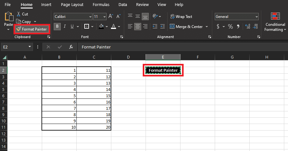
Click on the “Home” button at the top of your screen. Here, choose the “Format Painter” option in the “Clipboard” section.
Now click on the other cells to which you wish to apply the same format.

You will have two cells with the same format but different data. If you want to apply the format of one cell to the other cells, double-click on the “Format Painter” option and click on the cells individually to which you want to apply the same format.

Wrap Text and Add Line Breaks

If you are typing in a cell in Excel, you can write in the same line forever. This is because the text does not wrap down to the new line. This can impact the readability of the text, especially where there is a lot of data in the adjacent cells.

Here are the steps to wrap the text in a cell to enter the new line:

In your Excel, click on the “Home” option at the top of the screen.

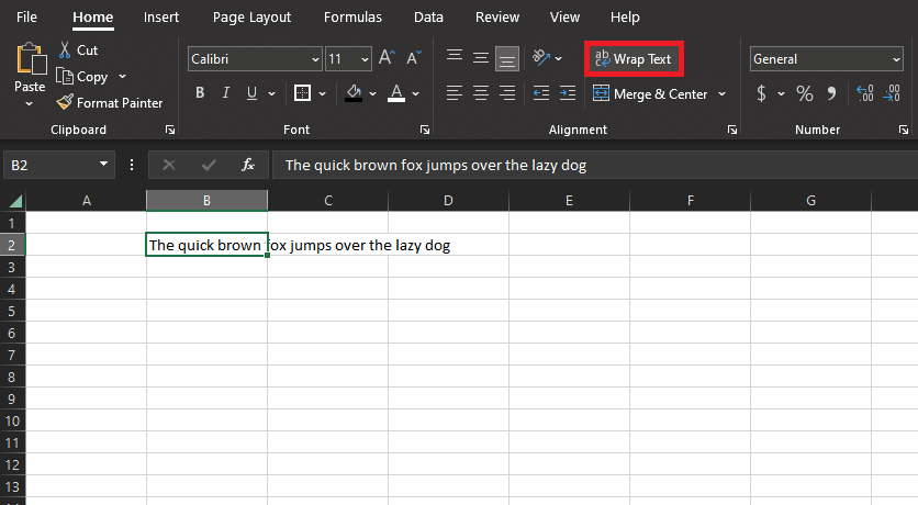
Now, choose the “Wrap Text” option. Your text will be wrapped in the corner of your selected cell. You can now resize your column or row, and the data in the cell will re-wrap to fit in it.
Another way to do this is by pressing your laptop’s Alt + Enter key.

If you want to wrap multiple cells with text overruns — select all the cells before clicking on the “Wrap Text” option. You can also select all cells using the Ctrl + A keyboard shortcut in your spreadsheet and choose the “Wrap Text” option so you do not have to manually do it later.

Autofill Cells

This feature is, by far, the best feature in Excel, as it is extremely useful in almost every type of spreadsheet. Let’s say you want to enter a sequence of numbers or dates into your Excel sheet following a pattern. Follow the steps below:

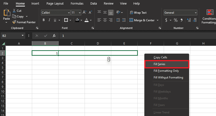
Instead of filling them out manually, write the first value of the series in the initial cell.
Move your cursor to the bottom right part of the cell, which will turn into a Plus (+) sign.
Click and drag the fill handle using the right-click and fill the cells.
Once you let go of the right-click, a drop-down list will open where you can select the fill type.

A faster way to autofill the cells in your Excel sheet is to hold the Ctrl button on your keyboard and then left-click on the bottom right part of the cell and drag-fill it. Doing this will always autofill the cells in the selection.

Autofit Rows and Columns

Having equally sized columns makes your Excel sheet look neat at the cost of a lot of wasted space. Let’s say you have one column containing addresses while another contains the city name.

The width of the address column is going to be much larger than the city one. Ensuring the columns and rows are sized appropriately to your data can make your spreadsheet more readable without sacrificing space. Here is how to autofit the columns and rows:

Press the Ctrl + A keys on your keyboard to select the data.
Click on the Alt + H-O-I letters on your keyboard. Your data will autofit into the columns automatically.
Click on Alt + H-O-A on your keyboard to autofit your rows.

You will be able to read the data in your cells instantly. However, you will still have to use the scrollbar to see the entire sheet. Here is an alternative way of doing this:

On your spreadsheet, click the “Home” button at the top of the screen.
Click on the “Format” option.
Choose the “Autofit Row Height” option or the “Autofit Column Width” option.

Smartly Fill Data Using Flash Fill

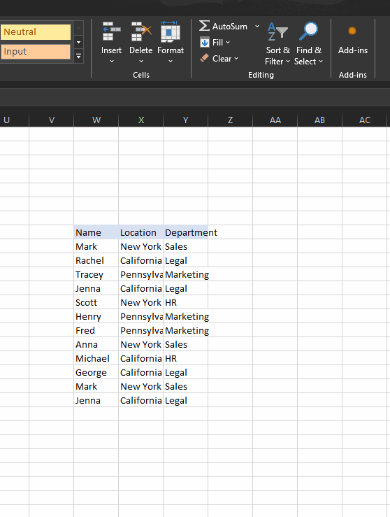
It’s helpful if the first row has a different header since “Flash Fill” will intelligently fill a column depending on the data pattern it detects in the first column.

For example, if you have written the phone numbers with 12124567890 and want to format them as 1-212-456-7890. Simply start entering the numbers with the new format. Excel will recognize the format and display it accordingly. All you have to do is press “Enter.”

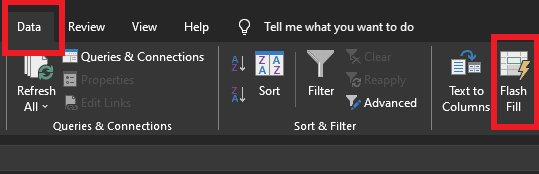
This applies to figures, dates, and names, too. Type in some more cells if the second cell does not provide you with a precise range; the pattern might not be obvious. Then click the “Flash Fill” option on the “Data” menu.

Select Data Using Ctrl + Shift

One of the fastest ways to select the data in your spreadsheet is by using the keys on your keyboard. Here is how to select your data:

Click the first cell in your spreadsheet that you wish to select.
Press and hold the Ctrl + Shift keys on your keyboard.
Depending on the data you wish to select, either press the left or right arrow key for selecting rows from your keyboard or the down or up arrow button for selecting columns.

One thing to keep in mind is that it will only select the cells containing your data. An alternative way of selecting data is to use the symbol. To do this, select the first cell containing the data and press the Ctrl + Shift + keyboard shortcut to select the data.

Text to Columns

If you have a column of names containing the forename and surname, and you want to break the column into two, here is how to do this:

Select the columns containing your data.

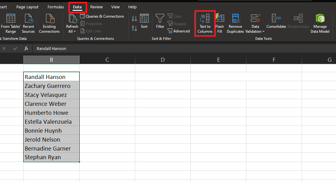
Excel column with a row of names—forename and surname

Click on the “Data” tab at the top of the spreadsheet and choose the “Text to Columns” option in the “Data Tools” section.

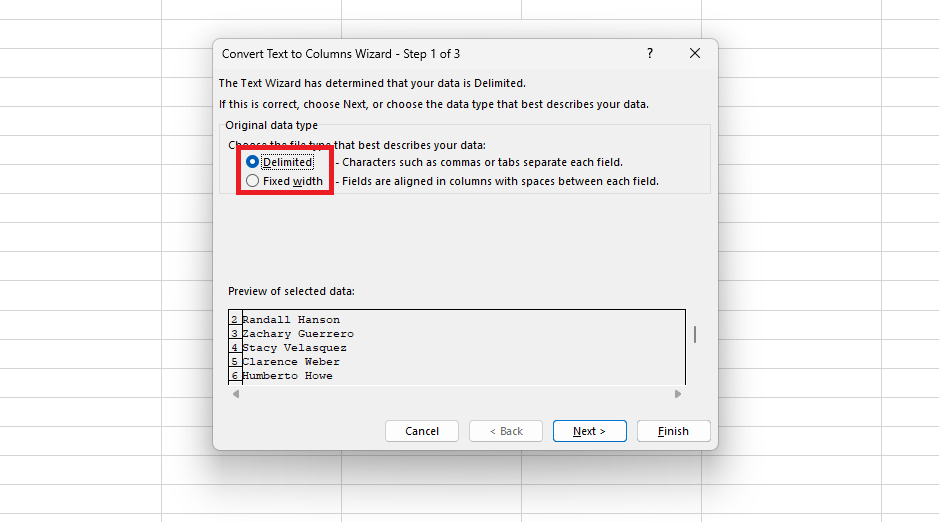
Excel Tips—Text to column wizard dialog box

This will open a window where you can choose the method you wish to use to split the data. The “Delimited” method is great if you want to split names, while the “Fixed Width” option is better suited for numbers. Click on “Next” after choosing your desired method.

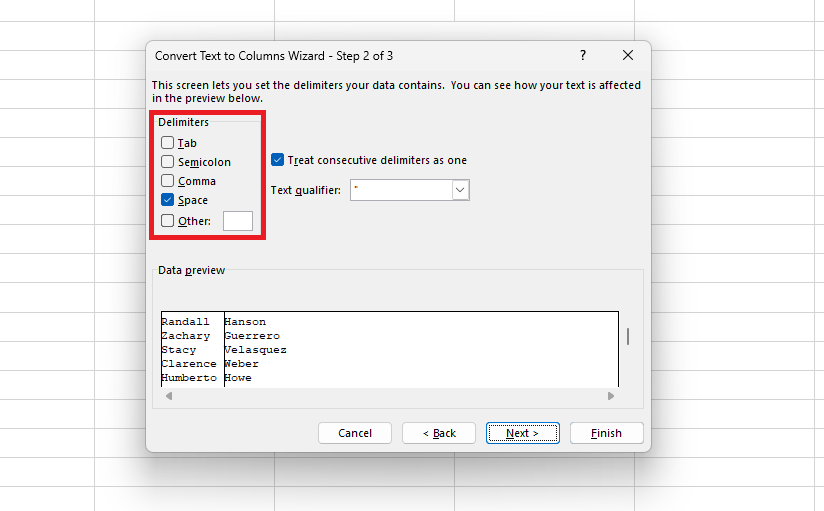
In the next section, you can specify the “Delimiters.”
- In this example, we are using spaces are they are used to separate the forenames and surnames.
- Click “Next” to go to the next section.

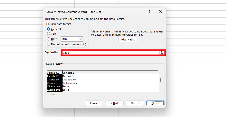
Delimiter option to separate forenames and surnames.

Specify the destination of the text.
- You can do this by entering the cell address or selecting it by pressing the arrow icon towards the right side of the textbox.

Paste Special to Transpose

If you have several rows and want to turn them into columns, it is very time-consuming to manually change your row data into the column data one cell at a time. By comparison, the method below saves a ton of time.

Here is how to change rows into columns:

Copy the row with the data that you want to turn into columns.
Click on the cell where you want to pull data from.
- If you’re transposing a column to a row, then the selected cell will be at the leftmost cell.
- If you’re transposing a row to a column, then the selected cell will be the topmost cell.

Click on the “Home” option in the main toolbar towards the top of the screen.

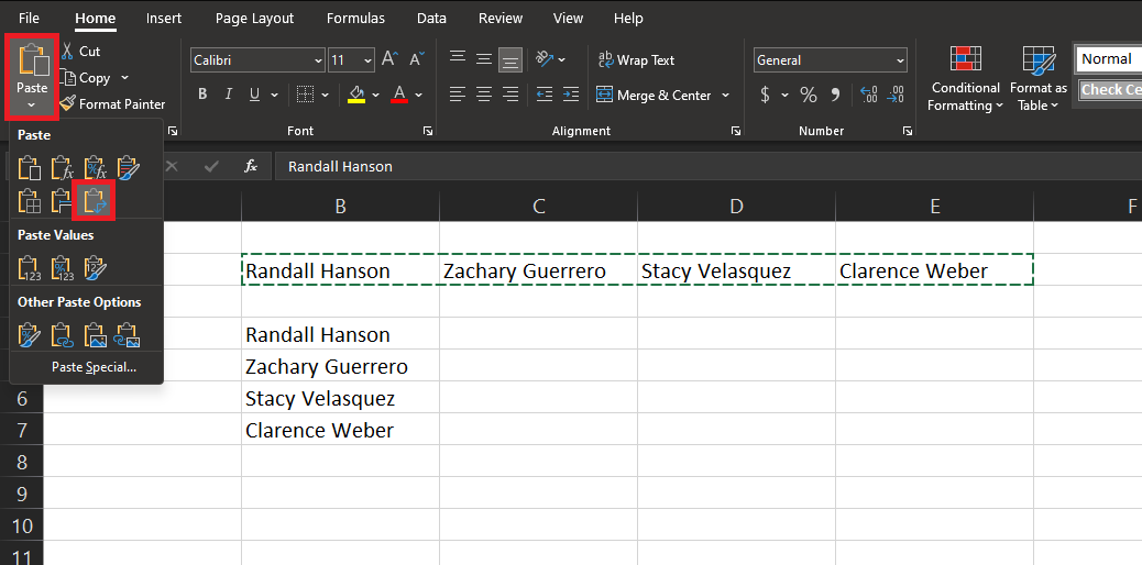
Choose the “Paste” option and click on the “Transpose” option.

Same Data on Multiple Cells

If you want to pull the same data, including formulas, into different cells repeatedly, this is an easy way to copy your data into multiple cells. Here are the steps to type the same data into different cells:

Click on the cells where you want to enter your data.
- You can do this by selecting the cells individually using the Ctrl key from your keyboard.
- You can select multiple columns or rows using the Ctrl + Shift + Arrow keys.

After you are done selecting, type in your data in the formula bar.
Press the Ctrl + Enter keys from your keyboard to enter the data into all the selected cells.

Hide Entire Worksheet

The file you’re working on may contain many worksheets, each denoted by a tab at the bottom and can be given a name. Instead of deleting a sheet, you can hide it so that its data is still accessible to formulas on other pages in the workbook and can be used for reference.

To hide the worksheet:

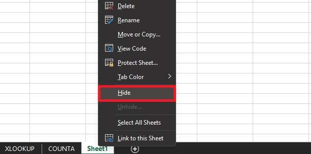
Right-click on the sheet you wish to hide. This will open a pop-up menu.
Choose the “Hide” option.
Alternatively, you can also do this by heading to the “View” tab using the main toolbar and clicking the “Hide” button.

To unhide the spreadsheet, click on any worksheet’s name from the tab list. Click on the “Unhide” option to open a new window there. Here, click on the worksheet’s name and click on “OK.”

Save Charts as Templates

Excel contains a lot of default charts. However, it can be difficult to find a chart that fits your data. In such cases, Excel allows you to customize the chart, but creating a new one can be complicated because starting a complex chart from scratch requires you to remember a lot of menu paths.

If you know you will need a particular chart several times, you can save your chart as a template instead. Here is how to save your chart as a template:

Right-click on the chart that you want to save as a template. This will open a drop-down list.

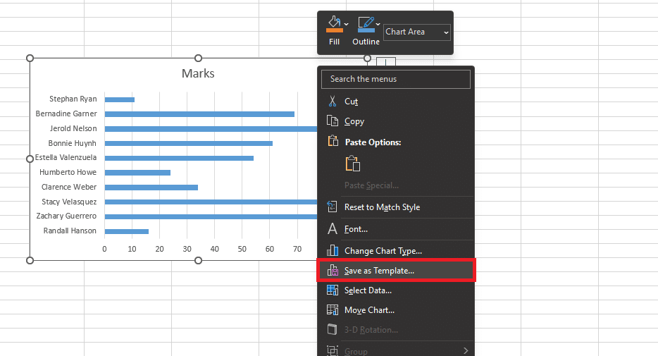
Click on the “Save as Template” option.
- You will be given the option to save the chart template file locally.
- Save the file with the CRTX version in a folder of your choice.

Select the data you want to turn into a chart and click the “Insert” option at the top of the spreadsheet.
- Choose the “Recommended Charts” option in the “Charts” section.

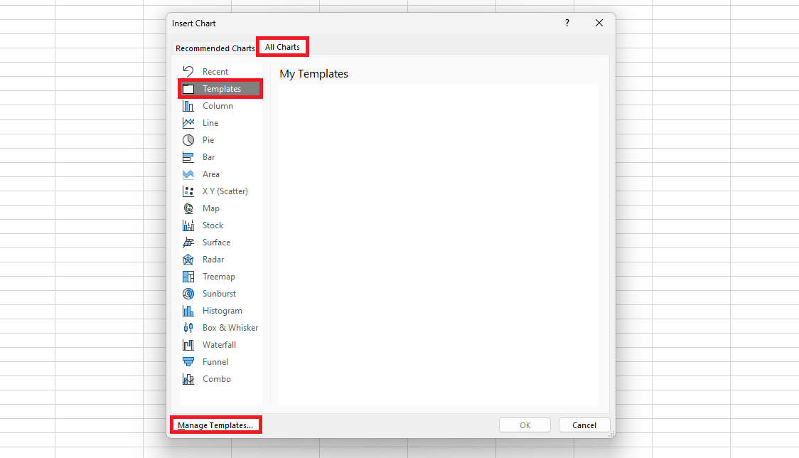
Click on the “All Charts” tab towards the top of the window and choose the “Templates” option in the sidebar.
Click the “Manage Templates” option towards the bottom left side of the window.
- This allows you to select the chart template file using the local browser.

Specific components, such as the text in the titles and legends, cannot be translated unless included in your selected data. But you can save options like fonts and colors, built-in graphics, and even series options, such as drop shadows.

If you’re looking for Excel templates, check out some of our spreadsheet templates. And don’t forget to use the promo code “SSP” during checkout for 50% off on all templates!

Get Premium Templates

Best Excel Keyboard Shortcuts

One great Excel tip for users is to learn the keyboard shortcuts and integrate them into your daily workflow. Keyboard shortcuts allow you to perform tasks faster than the mouse, reducing the time it takes to navigate, select, and manipulate data.

By using shortcuts, you can maintain a seamless workflow without interrupting your typing or data entry process to reach for the mouse. Additionally, keyboard shortcuts minimize the strain on your hand and wrist, promoting better ergonomics, as overusing the mouse can lead to repetitive strain injuries.

Here are some of the best shortcuts for Excel in 2024:

Creates a new worksheet: Ctrl + N
Opens existing worksheet: Ctrl + O
Saves current workbook: Ctrl + S
Closes current workbook: Ctrl + W
Move to the next worksheet: Ctrl + Page Down
Move to the previous worksheet: Ctrl + PageUp
Add a comment: Shift + F2
Find and replace: Ctrl + H
Insert hyperlink: Ctrl + K
Select the entire row: Shift + Space
Select the entire column: Ctrl + Space
Delete a column: Alt+H+D+C
Delete a row: Shift + Space, Ctrl + –

These are just a few shortcuts for some of the most basic tasks you will perform in your spreadsheet.

However, you can also create your own custom shortcuts by clicking on the “File” tab and then on “Options.” There, in the window that shows up, head over to the “Advanced” tab and scroll to find the “Keyboard Shortcuts” section. Here, you can click the “New” button and add the desired key combination.

Related Reading: 20 Google Sheets Shortcuts You Must Know!

How To Use Formulas in Microsoft Excel

An Excel formula is an expression that can be used to perform calculations, carry out specific functions, or manipulate the data in your spreadsheet.

Currently, there are more than 475 formulas in the function library. All formulas follow the same pattern. Let’s take a look at the pattern before we look at some of the most useful formulas in Excel:

= FunctionName (Parameter,Parameter)

Equals Sign (=): This initializes a formula. It tells Excel to treat anything after the sign as a function. Without this, Excel will treat your formula as regular text.
Function Name: This is the name of the built-in function in Excel. Entering the name will also autofill the formula telling you the parameters needed for the formula to work.
Brackets ( ): The opening and closing brackets group the operations together. When added after the Function Name, you can add the parameters for the function inside the bracket. If brackets are used outside of a function, they will essentially create groups that Excel will prioritize.
Parameter: The parameters in a formula refer to a variable or a value that you can input in the formula of the function in order to perform a calculation.

Now that you know how formulas work, let’s take a look at some of the top Excel formulas for 2024.

Excel SUM Function

The SUM formula is a basic yet one of the most powerful formulas in Excel. The primary purpose of this formula is to add up large sets of data.

Using the SUM function, you can easily calculate the total for columns, rows, or even a two-dimensional table. Here is the syntax of the SUM formula in Excel:

=SUM(val1, val2, …)

The function requires you to specify at least one val parameter for the formula to work. You can have up to 255 optional val parameters.

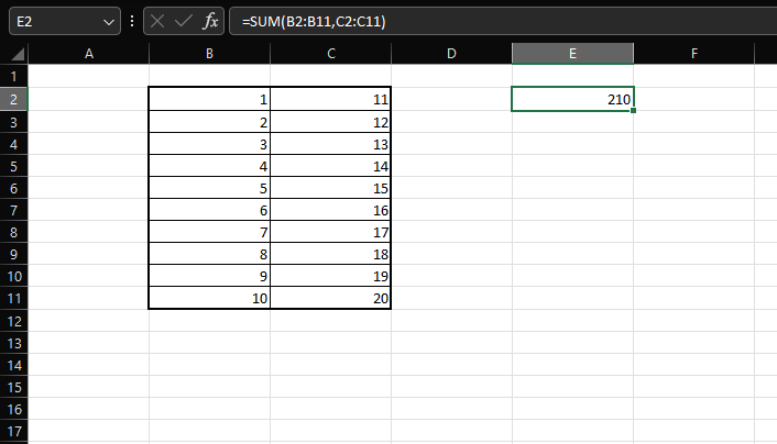
As an example, assume that we have two columns that contain a total of 20 values, which we want to sum up and show in another cell. The formula is written as:

=CONCATENATE(C2, ", ", B2)

Excel CONCATENATE Function

The CONCATENATE is another great Excel function that allows users to combine text from multiple cells into a single one. Not only that, but you can also add extra characters within the text.

This is a great formula to use for data manipulation as well as the organization of data. Here is the syntax of the CONCATENATE formula in Excel:

=CONCATENATE(txt1, txt2, ...)

The function requires you to specify at least one txt parameter for the formula to work. You can have up to 255 optional txt parameters.

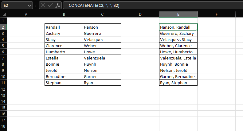
As an example, assume that you have two columns. One contains the first name, and the second contains the people’s last names. We want to write the surname first and the forename afterward, with both names separated by a comma. The formula is written as:

=CONCATENATE(C2, ", ", B2).

Excel IF Function

The IF function in Excel performs a conditional test on the given data and then returns predefined values based on the result. It can help automate any decision-making processes without the user having to do them manually. Here is the syntax of the IF formula in Excel:

=IF(test, true-val, false-val)

The formula requires two parameters to work. The first is the test parameter, where you will define the condition you want to check for. The true-val parameter is the value that will be returned if the test result is true.

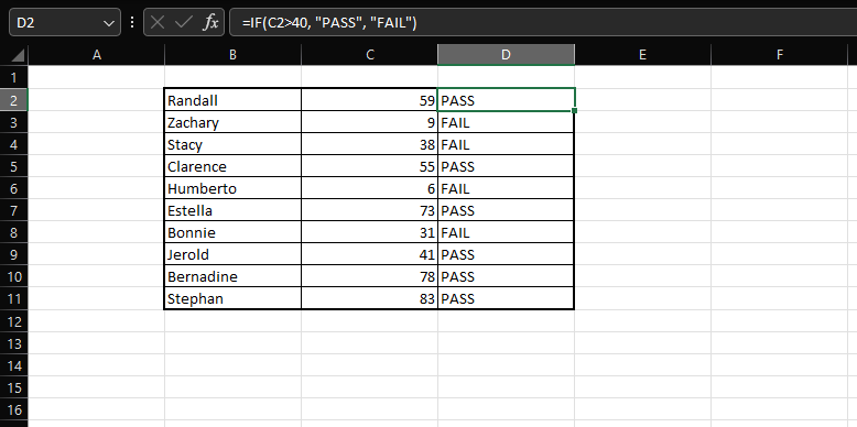
For example, let’s say we have a column containing the students’ marks in a class, and we want to write whether the student is PASS or FAIL automatically. The formula is written as:

=IF(C2>40, "PASS", "FAIL")

Excel AVERAGE Function

The AVERAGE function in Excel calculates the mean value of multiple numbers or a cell range. This function allows you to simplify the data analysis process as it provides a quick way to find the average value and allows the user to understand the trends, performance, and other characteristics of the spreadsheet easily and efficiently.

Here is the syntax of the AVERAGE formula in Excel:

=AVERAGE(val1, val2, …)

Similar to the SUM function we discussed before, AVERAGE requires you to specify at least one val parameter for the formula to work, and you can have up to 255 optional val parameters.

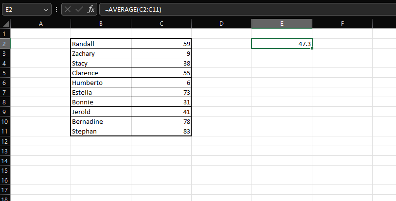
Taking the same example as before, let’s say we want to find out the average marks of the students in a class. The formula for AVERAGE will be written as

=AVERAGE(C2:C11)

Excel COUNTA Function

The Excel COUNTA function tallies the number of non-empty cells within a given cell range, counting all cells containing text, numbers, dates, and logical values.

It helps analyze data completeness, identify blanks, and obtain the total count of populated cells, aiding in data validation and decision-making processes. Here is the syntax of the COUNTA formula in Excel:

=COUNTA(val1, val2, …)

Like the other functions we discussed above, the function requires you to specify at least one val parameter for the formula to work. You can have up to 255 optional val parameters.

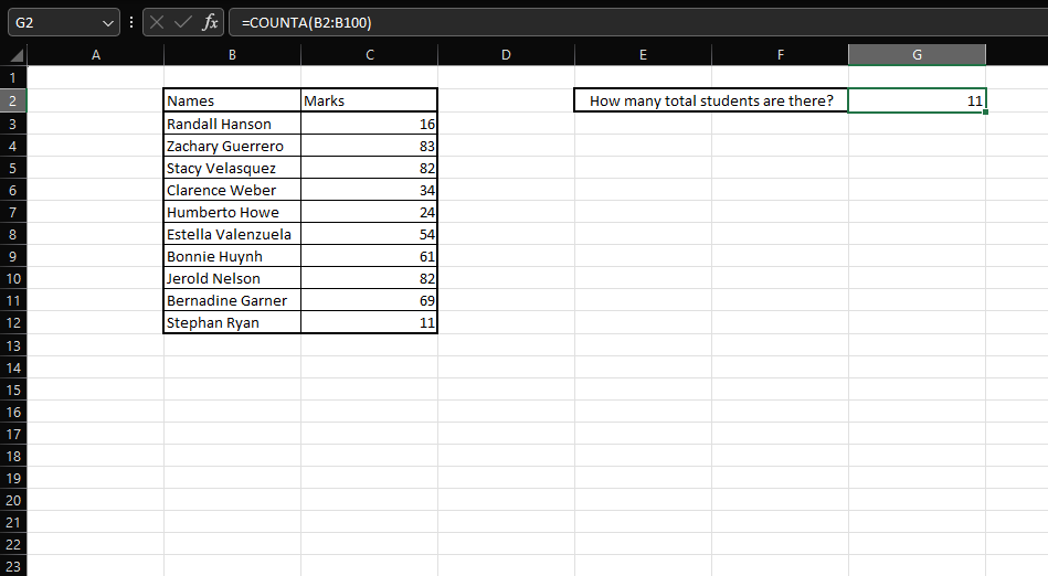
In this example, let’s say we have a list of students we want to count and display the total number that dynamically updates when new students are added. The formula for COUNTA will be written as:

=COUNTA(B2:B100)

Note: The cell reference is larger than the total number of students. However, COUNTA will ignore all the blank cells. This means you can select more cells in a column if you intend to add more data later.

Excel SUBSTITUTE Function

The Excel SUBSTITUTE function replaces different occurrences of a specified substring within a text string with a new substring. It allows users to substitute one or all occurrences, making data manipulation and formatting tasks more efficient.

This function helps clean data, modify text, and perform various text operations in worksheets. Here is the syntax of the SUBSTITUTE formula in Excel:

=SUBSTITUTE(text, old, new, instance)

The formula requires at least three parameters to work properly. The parameters are:

text – This required parameter defines the text or the reference to the cell containing the text you want to substitute with the new text.
old – This required parameter defines the text you want to replace.
new – This required parameter defines the text you want to replace the old text with.
instance – This optional parameter defines the number of occurrences of the old text you wish to replace with the new text. If this parameter isn’t defined, every occurrence of the old text is replaced with the new text.

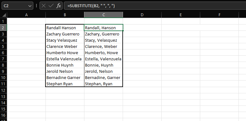
For example, let’s say we have full names, and we want to change the format so that they are separated by a comma instead of a space. The formula for SUBSTITUTE will be written as:

=SUBSTITUTE(B2, " ", ", ")

Excel XLOOKUP Function

The XLOOKUP function in Excel is an easy-to-use reference function that allows the user to efficiently find and fetch data from the specified cells. This simplifies the data search as it supports exact and approximate matches, providing exceptional flexibility for the user.

XLOOKUP is not available in Excel 2016 and 2019. However, the formula can still work if a file is opened from the newer Excel version. Although other alternate functions like VLOOKUP and HLOOKUP are still usable in Excel, we recommend using the vastly improved XLOOKUP.

Here is the syntax of the XLOOKUP formula in Excel:

=XLOOKUP(xlook-val, xlook-array, ret-array, not-found, match, search)

The formula requires at least three parameters to work properly. The parameters are:

xlook-val – This is a required parameter that is the value you want to search for in the xlook-array parameter. This value can be input directly into the function or add a cell reference.
xlook-array – This required parameter defines the cell range where you want to look for the value defined in the xlook-val parameter.
ret-array – This required parameter defines the range or array you want to return.
not-found – This optional parameter defines the text you want to display if a valid match is not found. If this parameter is not defined, the formula will return #N/A.
match – This parameter is also optional and defines the match type. This can have one of the following values:
- 0 – This value will show an exact match and is the default for this parameter. If no match is found, then the not-found parameter is displayed.
- -1 – This value will also return an exact match. However, if no match is found, Excel will return the next smaller value.
- 1 – This value will return exact matches. If none are found, then the next larger value will be output.
- 2 – This is a wildcard match where you can use ?, *, and ~ to define the parameter.

search – This parameter defines the search method you want to use. This parameter can have one of the following values:
- 1 – This value will perform a lookup starting with the first item. This is the default value for this parameter.
- -1 – This value performs a reverse search starting at the list’s last item.
- 2 – This parameter will perform a binary search based on the XLOOK-ARRAY sorted in ascending order. If the sorting is incorrect, then unexpected results may be returned.
- -2 – This parameter will perform a binary search based on the XLOOK-ARRAY sorted in descending order. If the sorting is incorrect, then unexpected results may be returned.

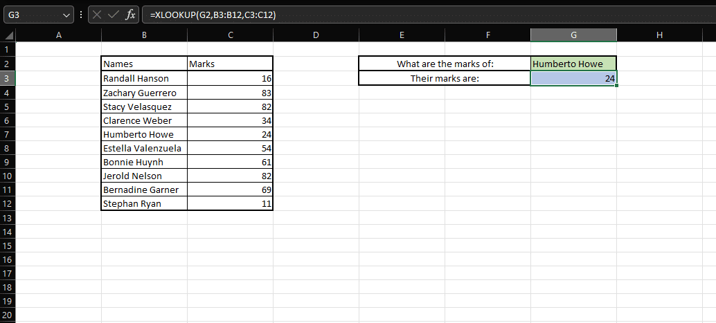
Let’s take a look at an example of the XLOOKUP function in action. In this example, we want to get the marks of a specific student by typing in their name. We will designate cell G2 as the search box. Cell G3 will be where the results are shown, and the formula will be entered. The formula for XLOOKUP will be written as:

=XLOOKUP(G2, B3:B12,C3:C12)

Mobile Excel Tips and Tricks 2024

Excel for mobile and Excel for Windows share many standard features and functionalities. However, there are also some differences in the user interface and the user experience between the two versions due to the varying platforms and device capabilities.

Here are some Microsoft Excel tips and tricks for mobile devices.

Typing Text Easily

Typing your text in a worksheet cell is quite different if you use Excel on Android or iOS.

The keys you are familiar with on your computer must be adjusted when using Excel on mobile. Below are a few Excel tips and tricks you can use when typing on mobile:

Here is how to type text in Excel:

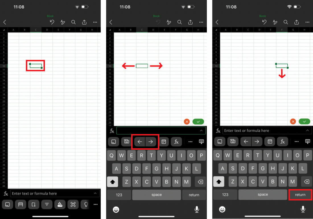
Excel - How to type in the mobile version

Open Excel and open a spreadsheet where you wish to make changes.
Double-tap on the cell you want to add text to. This will open your phone’s keyboard.
Enter the text using the keyboard.
You can use the Arrows above the keyboard in order to move the cell selection left or right to navigate the cells.
Click on the “Enter” or “Return” option on the keyboard to jump to the cell below.

Here is how to delete your Excel cell text:

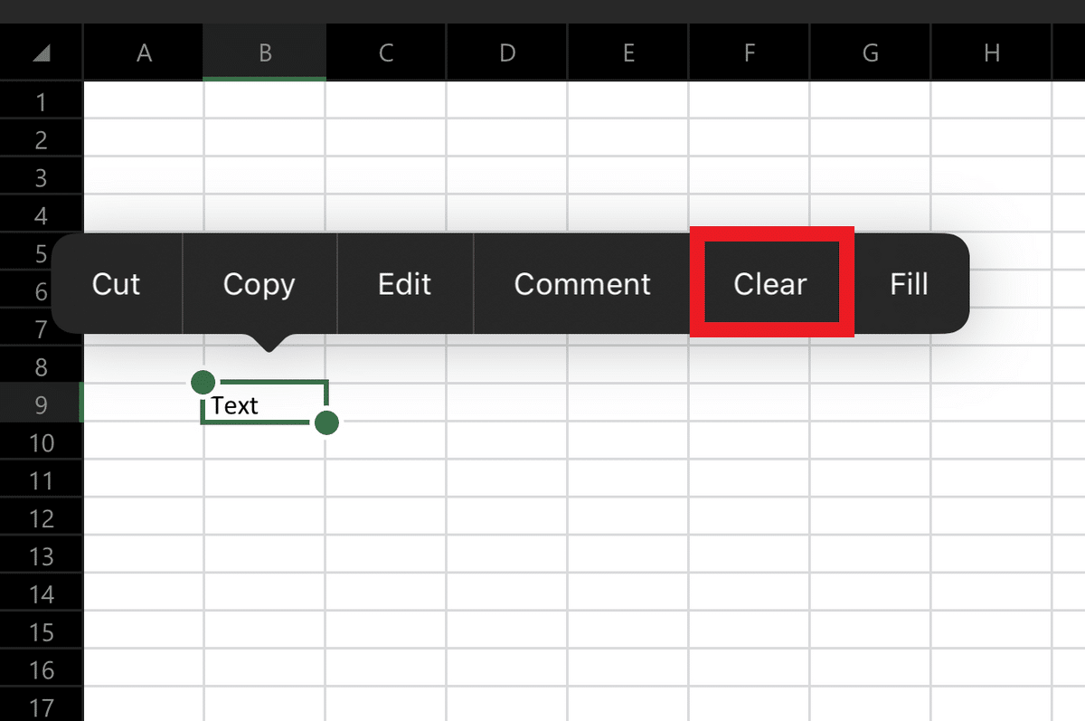
How to delete text in Excel's mobile version

Click a cell you want to delete to select it.
Tap and hold the cell for a few seconds until the context menu appears.
The menu will differ based on the phone’s OS and software skin. Here, click the “Clear” or “Delete” option.

Here is how to edit your cell text:

Double-click on the cell that you want to edit.
You will see a blue cursor; hold and drag it to where you wish to make the changes.

Creating Multiple Paragraphs

Writing multiple paragraphs or lines on both your desktop and your mobile is possible. However, for multiple paragraphs, you have to take a few extra steps on your mobile. Here is how to make multiple paragraphs in a cell:

Open Excel from your “Home” screen and head to the spreadsheet where you want to add the paragraphs.
Double-click a cell and start typing your text in.
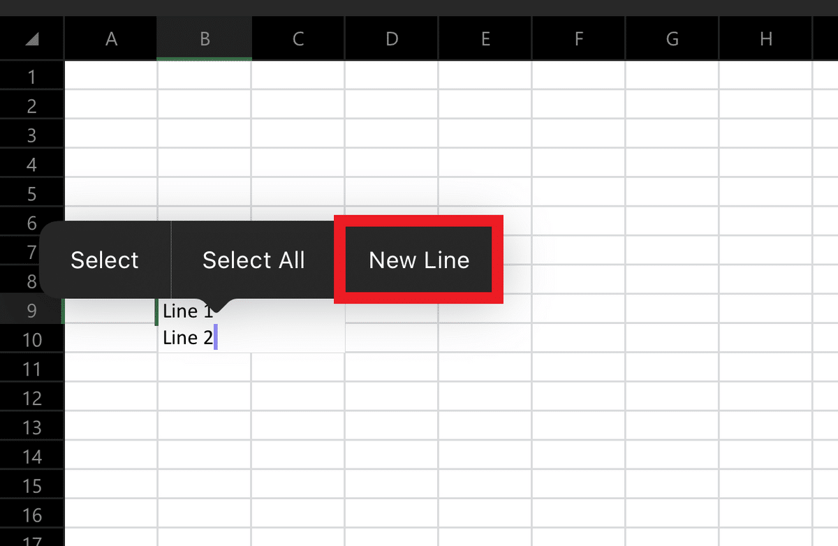
Once you are done writing the first line, click on the cell again and click the blue cursor when it appears.
In the “Context” menu that shows up, choose the “New Line” option.
Type in your text. Feel free to repeat steps 3 and 4 to add more lines.
When you are done typing in the cell, click on the green “Tick” icon on the right side of the screen above the keyboard.

Adding Numbers Quickly

One of the biggest use cases of Excel is to perform mathematical operations on numbers. If you want to add numbers of a row or a column on Android, you can use the “AutoSum” tool to add the numbers quickly.

Here is how to add your numbers:

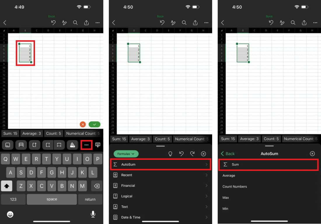
Excel's AutoSum option on mobile devices

Select the row or column with the numbers you want to add.
In the main toolbar, click on the “Ellipsis” icon above the keyboard.
Click on the “Formulas” option from the top header.
Choose the “AutoSum” option from the menu.
Click on the “Sum” option. The total will be displayed at the end of the column or row.

Using Filters for Sorting Data

If you want to organize the data on your Excel spreadsheet via a mobile device, you can sort it using the “Filter” tool. The tool allows you to sort the data in a numerical or alphabetical order. Here is how to use the filters:

On your Excel, click on the “Ellipsis” button on the screen’s right side.
Scroll down and choose the “Sort & Filter” option.
You can select the “Sort Ascending” or “Sort Descending” option to sort your data.

You can also click on the “Show Filter Buttons” option to show the “Filter” buttons in the spreadsheet’s top row. Click on the “Filter Button” from the column you wish to sort the data and choose a sorting option.

Drawing on the Spreadsheet

While drawing on a desktop with your mouse cursor is possible, your smartphone’s touchscreen makes it much easier for you to draw on your Excel spreadsheet.

Here, you can draw shapes like a circle or a line on your spreadsheet with your finger. Below are the steps to draw on Excel via a mobile device:

Click on the “Home” option from the left side of the screen and choose the “Draw” option.
Click on the “Draw with Mouse or Touch” option.
Click on the “Ink Color Selector” option.
Choose the thickness and color of the pen.
- Now, you can start drawing on your spreadsheet or change your pen color.
- If you want to use multiple colors for your drawing, click on the “Ink Color Selector” option and click on a different color or thickness.

Adding a Picture Using Camera

It is possible to add a picture directly on your Excel spreadsheet on mobile by using your phone camera. Here is how to insert a picture using your phone’s built-in camera:

How to add a picture via a mobile device

Open Excel from your “Home” screen and open the spreadsheet where you want to add the image.
Click on the cell where you want to add your picture.
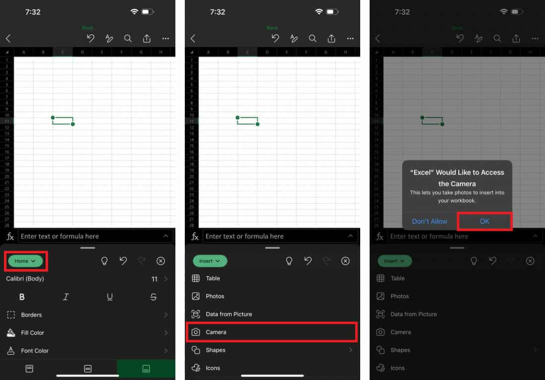
Click on the “Home” option in the toolbar and choose the “Insert” option in the drop-down menu.
In the “Insert” menu, click on the “Camera” option. Here, you can also add a photo from your phone’s gallery by clicking on “Photos.”
Take the picture and click on the “Confirm” option.
Click the “Done” option, and the picture will appear on your spreadsheet.

If you want to edit the picture, you will see the following editing options, like Crop Picture and Styles, within the “Picture” option.

Turning Data Into an Image

Suppose you want to protect your text in an Excel spreadsheet from changes. In that case, converting your data into a picture is the easiest way to save it from accidentally being changed or edited later. Here is how to convert your text into a picture:

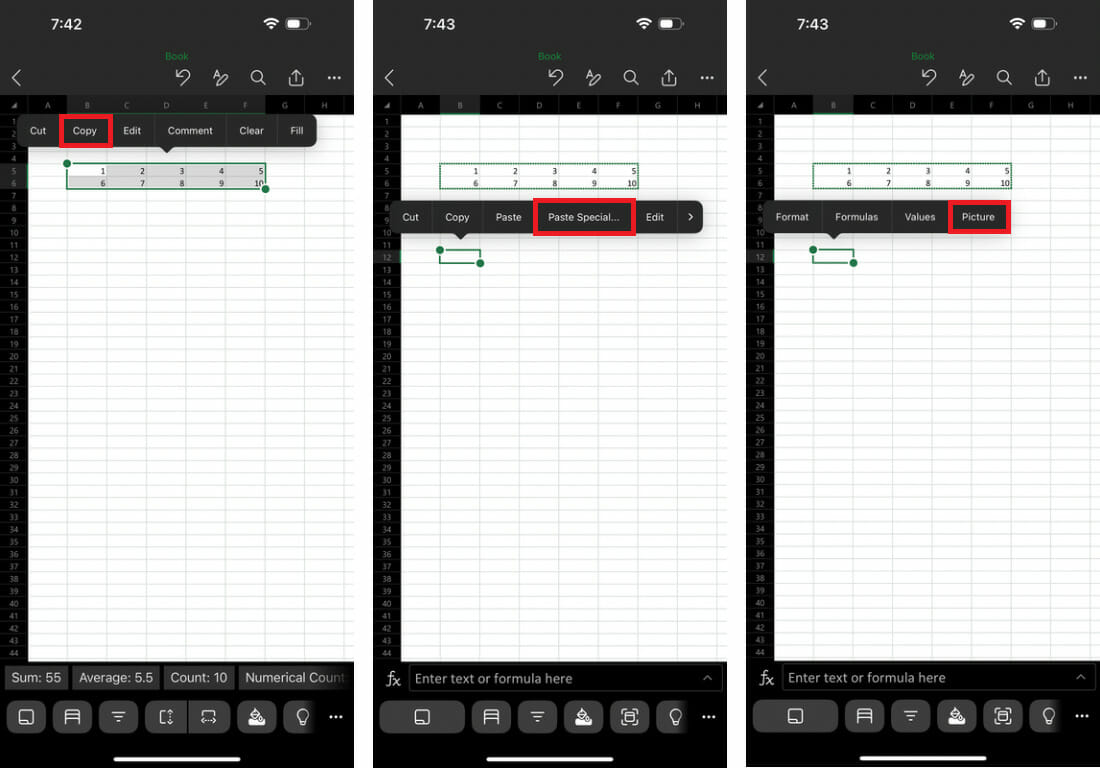
How to turn data into an image on Excel mobile

Select the text you want to turn into a picture.
From the “Context” menu, select the “Copy” icon.
Click and hold on to your cell where you want to paste your picture.
Go back to the “Context” menu and click on the “Paste Special” button.
From the “Paste” menu, choose the “Picture” option.

Here is an alternative way to turn data into an image:

Select the text and click on the arrow pointing downward.
Choose the “Picture” option from the “Paste” menu to convert your text into a picture without copying it anywhere else.

Using the Research Help

If you want to search the web using the Excel application on Android or iOS, using the “Smart Lookup” tool is the easiest way to research without leaving the Excel application. This tool helps you to find information, history, and definitions.

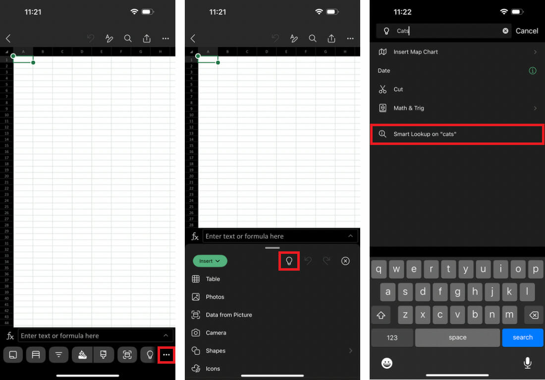
To use the Smart Lookup tool in Excel on mobile:

Click the “Ellipsis icon in the main toolbar towards the bottom of the screen.
Click on the “Bulb” icon towards the top part of the main header.
Type in your search term in the search bar and click on the “Smart Lookup on” button.

Adding Comments in a Spreadsheet

Adding a comment to a spreadsheet is useful if you want to ask a question or write a statement to your team working on the same project. Here is how to add a comment to a spreadsheet on mobile:

How to add comments in an Excel spreadsheet via mobile

Click on the cell where you want to add a comment and press the “Ellipsis” button in the toolbar.
Click on the “Home” option and choose the “Insert” option from the drop-down menu.
Scroll down and select the “Comment” option.
Type the text you want to write as a comment.
Click on the “Send” or “Post” icon on the screen’s right side.

Here is how to see your comment:

Click on the cell where you left the comment.
Click on the “Comment” icon on the cell’s right side.
After reading the comment, click on the “Cross” symbol to close it.

Sharing your Excel Spreadsheet

If you want to send your Excel spreadsheet to others, here is an easy way to share it on Excel for Android or iOS:

Open the spreadsheet you wish to share.
Click on the “Share” symbol at the top-right of the screen.
Here, you will see two options: A Workbook and a PDF. Click on the option of your choice.
Now choose if you wish to share it via email or any installed messaging app like WhatsApp or Messenger.

Creating Charts

If you want to add a chart for your data, the best way is to use the charts recommended in Excel to find one that fits well with your data.

Here is how to use charts for the representation of your data on Microsoft Excel for mobile:

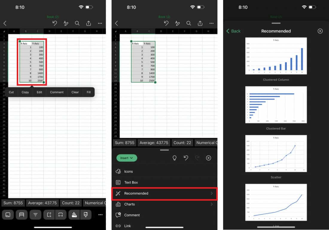
Find and highlight the data you want to use for making a chart.
- Ensure you also select the header labels, which will be used to label the X and Y axes.

Click on the “Ellipsis” icon, which will show the extended toolbar.
- You can skip this step if the extended toolbar is open.

Click on the “Home” option in the header and select the “Insert” option.
Scroll down and choose the “Recommended” option, which will recommend appropriate chart types according to your data.
Choose the chart of your choice from the recommended charts. The chart will appear on your spreadsheet, visualizing your selected data.

If you want to customize your chart, click on it, and under the “Chart” option, you will see the different editing options, such as size, layout, and color.

Creating Maps

If you want to convert your geographical data into a map, you can use the “Maps” option in Microsoft Excel for Android or iOS. Here is how to make a map:

Highlight the data you wish to make a map of and tap on the “Ellipsis” icon towards the right side of the toolbar.
Click on the “Home” option to open the drop-down list.
- There, click on the “Insert” option.

Scroll down and choose the “Chart” option.
Click on the “Maps” option and choose the type of map you want to add.
A confirmation menu will show up. Tap the “I agree” option, and the map will be added to your worksheet.

You can customize your map from the “Chart” option if appropriate.

Renaming Your Spreadsheet

Microsoft Excel assigns a simple name to your worksheets when you create them, making it hard to distinguish them from the other worksheets. Therefore, renaming multiple sheets helps you to identify your worksheet from many others saved in your workbook.

Here is how to rename your spreadsheet.

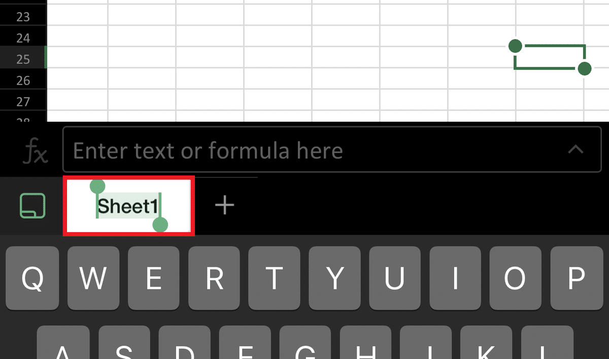
Click on the “Worksheet” symbol that is at the bottom-left side of the screen.
Double-click on the “Sheet 1” option.
Rename it with a name of your choice.
Click on any part of the spreadsheet to save it.

Hiding and Unhiding Rows

The process of hiding and unhiding rows in your worksheet on your mobile is similar to hiding them on your desktop. Hiding all the columns and rows that you don’t need on your spreadsheet can help with the organization of the spreadsheet and also make it look less cluttered.

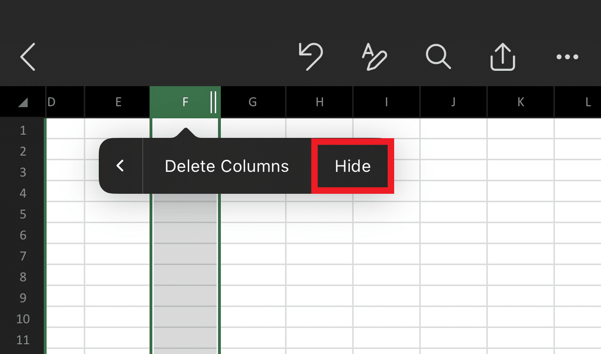
To hide the rows or columns on Android or ios:

Tap on the row or column header bar.
- The header bars for columns have numbers, whereas the header bars for rows have alphabets.

Tapping on the bar will show the “Context” menu.
Press the arrow icon to expand the options and click on the “Hide” button.

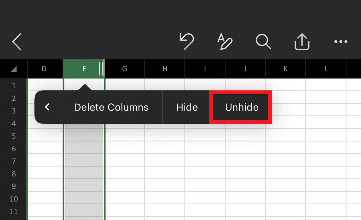
To unhide the hidden row or column, tap on any adjacent headers to show the “Context” menu. Press the arrow button to expand the options and tap on the “Unhide” option.

Frequently Asked Questions

How Can I Get Better at Microsoft Excel Fast?

To improve Excel skills rapidly, focus on learning key functions like VLOOKUP, tables, and other important formulas. Practice with real data and explore some of the advanced features like conditional formatting. Keyboard shortcuts and Excel courses online can also help you get better at Excel faster.

What Are the Five Basic Excel Skills?

The most basic formula you should learn to use is the SUM formula which helps you find the total values in your spreadsheet. Similarly, the AVERAGE formula provides the mean of the values you have in your spreadsheet.

Charts, graphs, and functions like conditional formatting make it easier to visualize numerical data. The Find and Replace feature helps you find a certain value in your spreadsheet. The Sorting Data feature helps you quickly interpret your Excel data and locate the necessary information.

How Can I Be an Expert in Excel?

You can become an expert by learning some Excel tips and tricks, as many shortcuts can make it easier to work on a spreadsheet. You should also learn the most popular Excel tools like Flash Fill and formulas and functions, such as the SUMPRODUCT and COUNTIF functions.

What Is the Hardest Function in Excel?

The difficulty of a particular function varies from one individual to another. However, most users find complex mathematical functions the hardest to master.

One such function is the CHISQ.INV.RT formula, which is used to return the inverse of the right-tally probability of a chi-squared distribution.

Is Microsoft Excel Easy to Master?

When it comes to organizing Excel data or spreadsheets, Excel can be difficult for beginners without prior knowledge. However, understanding the fundamentals is an easy starting point. People can learn the fundamentals of Excel through online classes in only a few hours.

Wrapping Up

By using the Excel tips and tricks we mentioned in this article, you’ll smash your way through spreadsheet creation quicker than ever. If you found this guide useful and would like to support our site, check out our premium templates, and remember to use the code SSP to save 50%.