The quickest way to learn how to collapse rows in Excel is to use the context menu by selecting the rows you want to hide and clicking “Hide.” Read on to learn how to do this by following the screenshots and learning the alternative ways you can collapse and expand rows in Excel.
Table of Contents
How To Collapse Rows in Excel
There are multiple ways that you can create collapsible rows in Excel:
Collapse Excel Rows Using the Context Menu
One of the easiest methods of collapsing or hiding a row is quickly removing all the data from your spreadsheet without deleting it. For example, if you have created a sales list and wish to hide some reps from your dataset. This easy process may work quickly, but it might not be suitable for a larger dataset.
Here is how to create collapsible rows in Excel using the context menu:
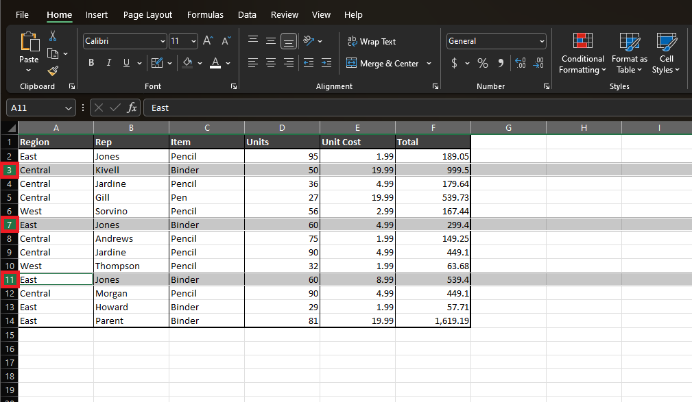
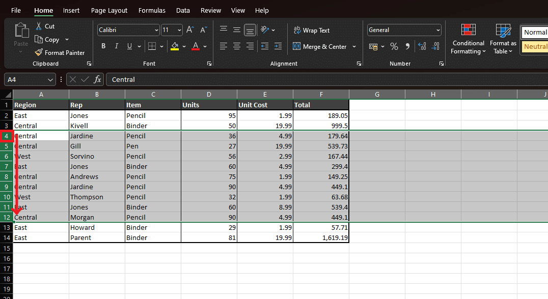
- Choose the rows you wish to hide by clicking towards the left side of the screen on the number bar. This will highlight the row in your spreadsheet.
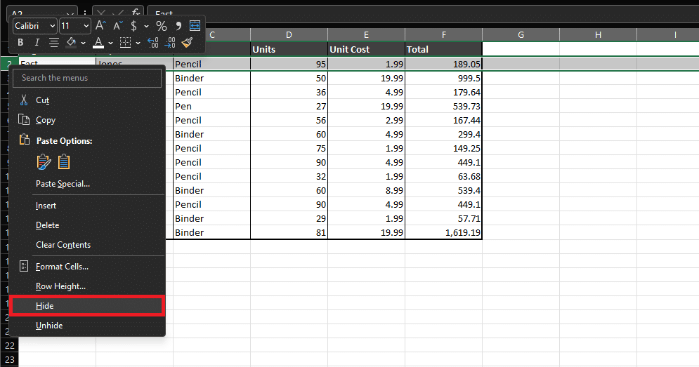
- Right-click on the selected row and click the “Hide” option from the context menu. Excel will automatically hide the selected row.
How To Expand Collapsed Rows in Excel
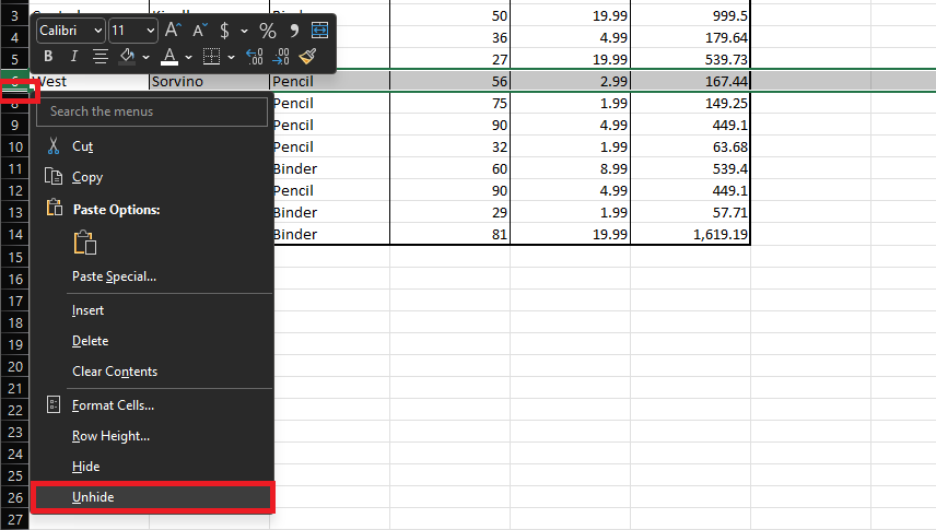
To view the hidden rows again, right-click on the number above the hidden row and choose the “Unhide” option.
Collapse Using the Group Feature (Collapse and Expand to a Certain Level)
The grouping feature can be used if you have similar categories of data. This way, you can create a group of rows that work similarly. You can combine all similar elements into one group, which can be easily collapsed. This makes it easier to hide or collapse your group with just a click.
Here is how to group and hide your rows in Excel:
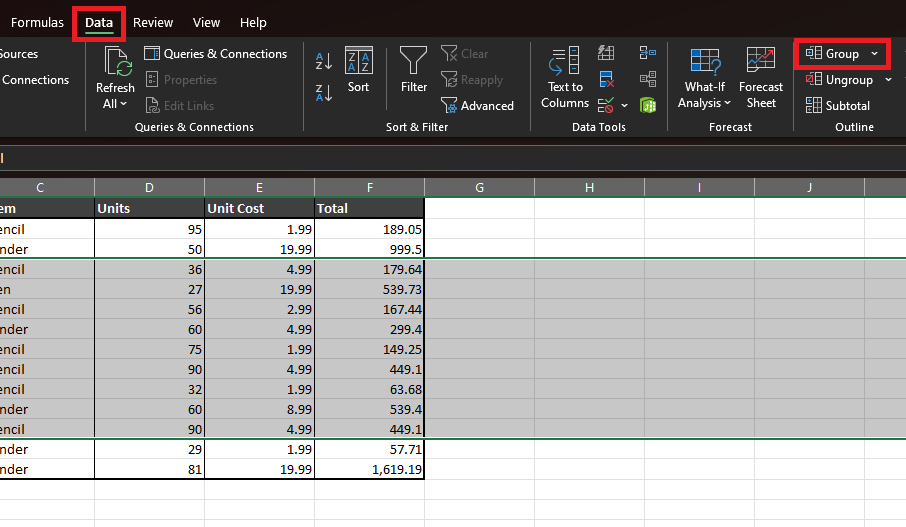
- Select all the rows you wish to make a group of.
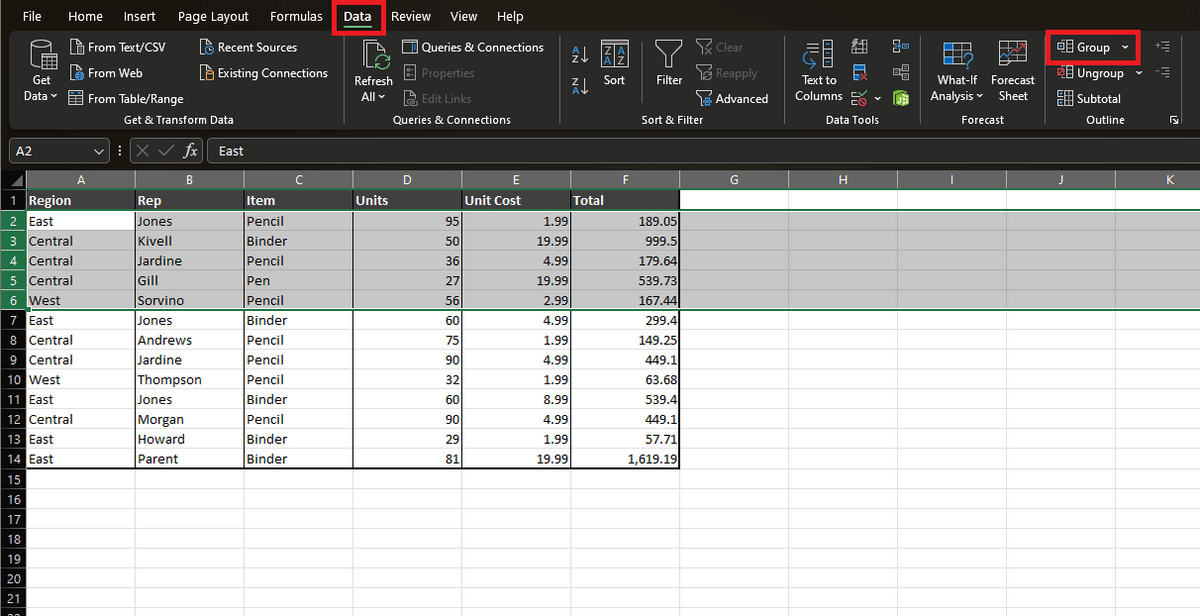
- Go to the “Data” tab at the top of the spreadsheet.
- Here, choose the “Group” option. Excel will automatically group all the selected rows together.
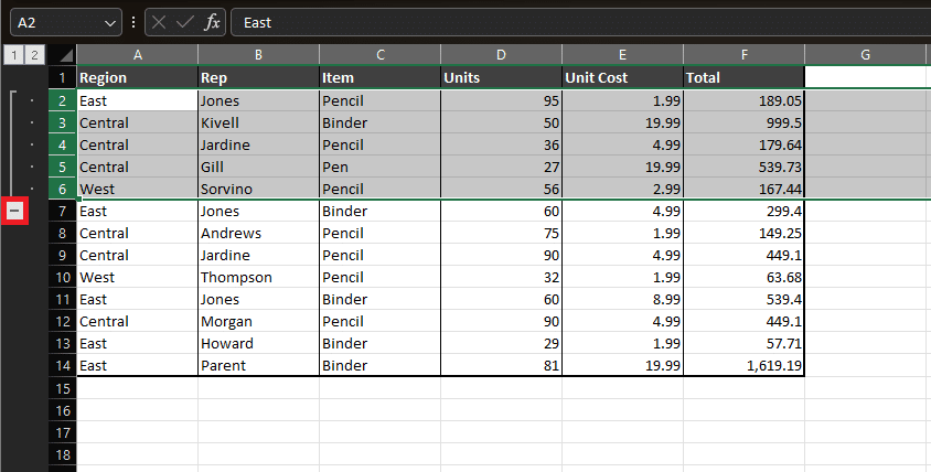
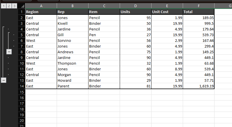
- To collapse the rows, click the Minus ( – ) icon in the side number bar.
How To Clear Collapsed Rows in Excel Using the Data Menu
Here is how to clear collapsible rows in Excel:
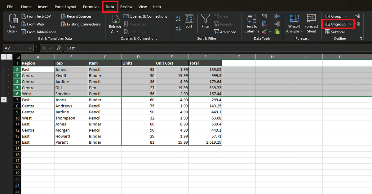
- On Excel, click the “Data” option at the top of the spreadsheet.
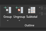
- In the “Outline” section, click the arrow beside the “Ungroup” option.
Excel will start clearing your collapsed rows from the outer to the inner levels. You will see at the top-left side of the spreadsheet that the level buttons have started to disappear.
Related: Can Google Sheets Group Rows and Columns? Yes, Here’s How
Collapse Using the Subtotal Feature
The subtotal feature is useful if you wish to create a group with a larger dataset by specific criteria. This way, you can create different groups by specific criteria like category or price. It can simplify the categorization of your data while providing a total for grouping.
Here is how to collapse groups with certain criteria in the overall data:
- Highlight the data by clicking and dragging the rows. Alternatively, you can click on the icon at the top of the numbers on the left.
- Choose the “Data” option from the top ribbon of Excel.
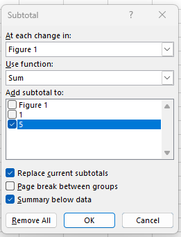
- Click on the “Subtotal” option from the sub-menu in the “Outline” group. This will open a small window where you can specify the row or column where you want to show the count.
- Check the box next to your desired option and click the “OK” option. Your data will now be in groups with their specific categories.
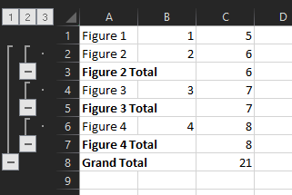
To hide and unhide your data, click on the Minus ( – ) or Plus ( + ) icons on the left side of your spreadsheet.
Collapse Using Filtering
You can use filtering to make complex spreadsheets with numerous categories or data sources invisible. This makes it much simpler to organize data into similar categories. Here is how you can collapse your data using filtering:
- Click and drag your cursor across the data set to select the desired data.
- Click the “Data” option from the top of the spreadsheet in the main menu bar.
- Click on the “Filter” option.
- Click the arrow at the top of any row.
- Select a type of filter and fill in how you want it to work.
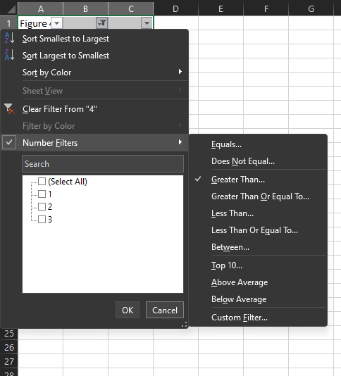
- Excel automatically collapses the rows that don’t meet the requirement requirements.
Collapse Using Row Height
This method is a manual way of collapsing or hiding rows. Even though it is useful to collapse the data quickly, you may find it difficult to rectify the rows. You can easily remove incorrect entries from the spreader using this method. Here is how to collapse the rows using the row height feature:
- Select the rows that you wish to collapse.
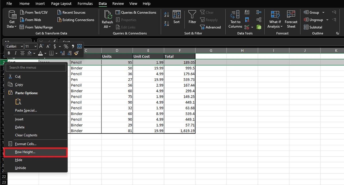
- Right-click on the selected rows and click the “Row Height” option.
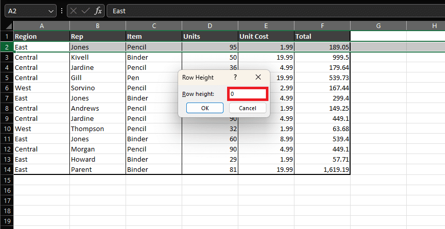
- Set your row height and type “0” in the box.
- Click on the “OK” option. Excel will automatically set the row height to 0, collapsing the selected rows.
To uncollapse the row, repeat the steps and set the “Row Height” to your chosen number. The default height for the row is 15.
Collapse the Rows Using the Home Tab
Using the “Home” tab is another easy way to collapse columns or rows. This method is similar to the Context Menu method but provides more options. Here is how to create collapsing Excel rows using the Home tab:
- Click and select the columns or rows you wish to collapse.
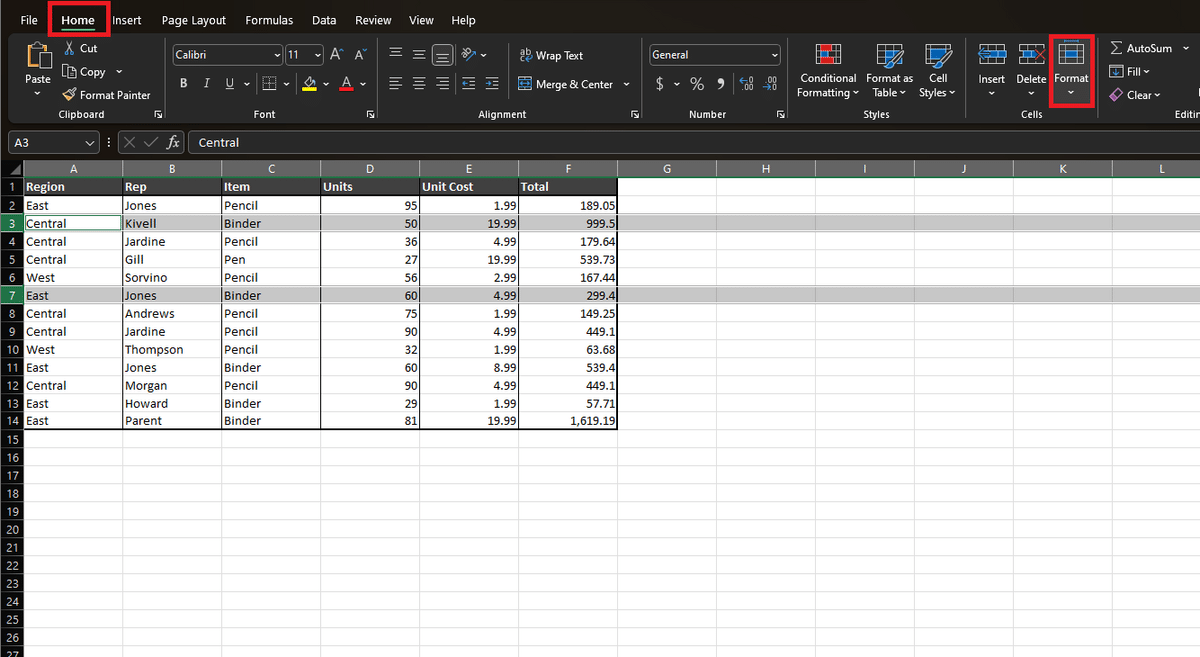
- Choose the “Home” option from the main toolbar.
- Now, click the “Format” option in the “Cells” section.
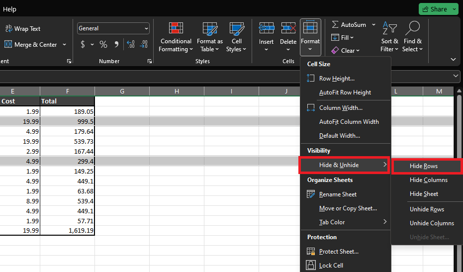
- In the “Visibility” section, click on the “Hide & Unhide” option.
- Click on the “Hide Rows” option in the pop-out menu. Excel will automatically hide the selected rows.
To reverse the Excel collapsed rows, follow the abovementioned steps and click on the “Unhide Rows” option in the pop-out menu.
Related: How To Unhide Rows in Google Sheets (7 Easy Examples)
Collapse Using Excel Keyboard Shortcuts
The keyboard shortcuts make it easier to work on your spreadsheet with a large dataset. Here are some helpful keyboard shortcuts for collapsing Excel rows:
- Hiding Groups: Alt + A + H
- Unhiding groups: Alt + A + J
- Select One Column or Row: Shift + Space
- Select Entire Spreadsheet: Ctrl + Space
How To Create a Nested Collapse in Excel
Microsoft Excel allows you to collapse the rows and columns in your spreadsheet. Not only that, you can create nested collapsible rows. Here is how you can create a nested collapse in Excel:
- Click and drag your cursor on the number bar (left part of the screen) to highlight the rows you want to create a collapsable group. In this example, we chose rows 4 to 12.
- Now, click on “Data” > “Group” > “Outline.” This will create the first group.
- Click and drag your cursor again to select the cells you want to add to the group you created in the previous step. In this example, we are going to choose rows 5-7.
- With the new rows selected, repeat step 2. Then, go to “Data” and click the “Group” button to create another group.
You can keep repeating the abovementioned steps to create multiple nested groups that allow you to sort your data easily. One example of using this method is if you have sales data for three years. You can create the first collapsable group for separate years. Then you can create a nested group for the year for every month.
Related: Google Sheets vs. Excel – Which Is Better In 2024?
How To Copy the Visible Rows in Excel
When working on your worksheet, you may not want to select data from the hidden rows in Excel. Here is how to copy and paste data from the visible rows:
- Select the rows you wish to copy.
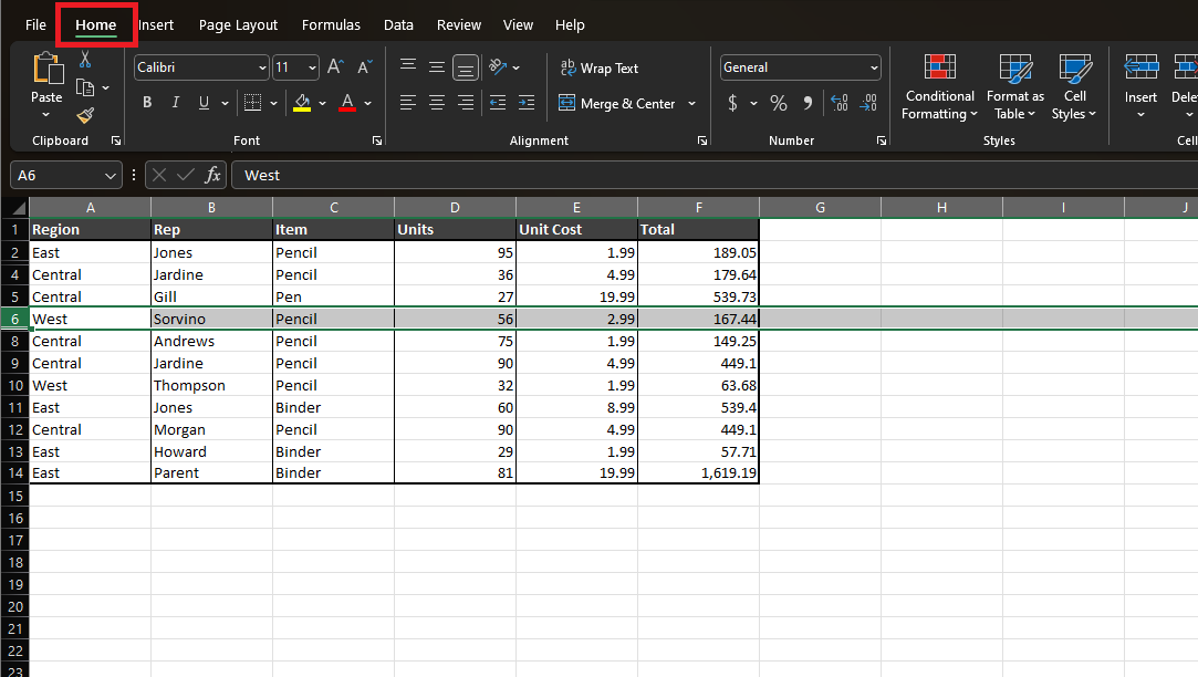
- Click on the “Home” option at the top of the spreadsheet.
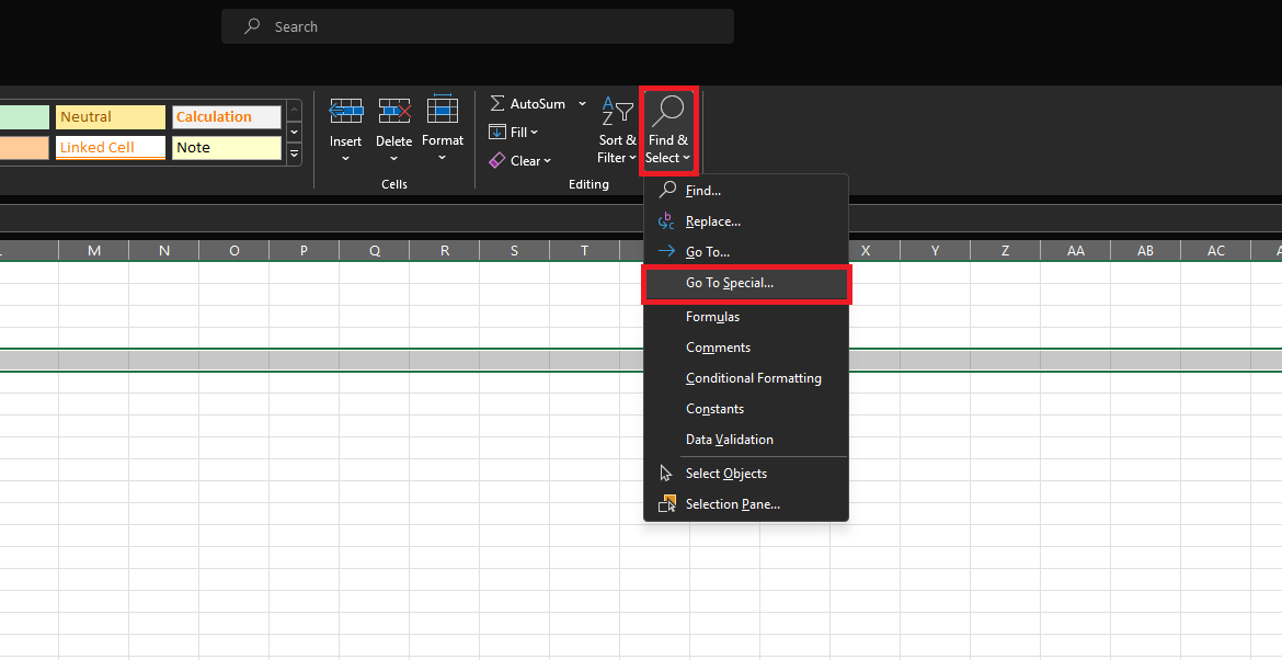
- Choose the “Find & Select” option on the spreadsheet’s right side.
- Click on the “Go To Special” option.
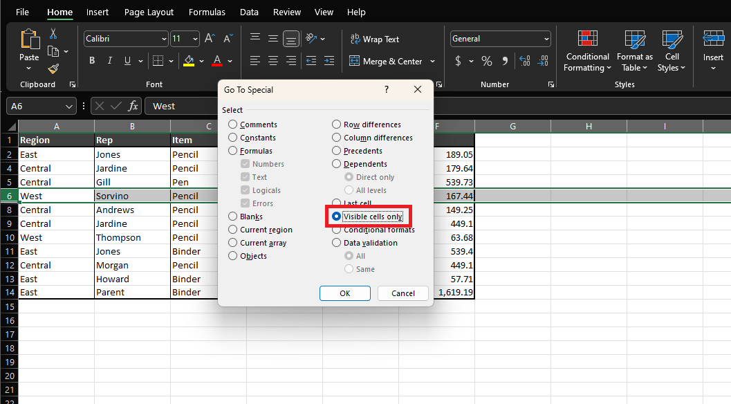
- Select the “Visible cells only” option.
- Click on the “OK” option.
- You can right-click on the highlighted rows and choose the “Copy” option or press the Ctrl + C keys from your Windows keyboard to copy the visible rows.
- Go to your desired location to paste the copied cells, right-click on it, and choose the “Paste” option.
Related: 11 Best Excel Courses Online in 2024
Frequently Asked Questions
What Is the Shortcut for Collapse Rows in Excel?
To collapse rows in Excel, select the data you want to collapse and press Alt + A + H keys from your Windows keyboard to hide the group.
What Is the Easiest Way to Collapse Rows in Excel?
The easiest way to collapse rows in Excel is to select the rows that you want to collapse. Simply right-click on the number bar at the left side of the spreadsheet of the highlighted rows and choose the “Hide” option from the drop-down menu.
To unhide the rows, repeat the steps and click the “Unhide” option.
How Do You Collapse Rows in Excel?
Select the rows you wish to make a group of and click the “Data” option. Select the “Group” option to make the group of the selected rows.
Now, you can click the Minus (-) icon in the side number bar to collapse the rows.
Wrapping Up
Although we’ve shown you how to collapse rows in Excel in many different ways, you’ll likely use the “Context Menu” most of the time. So, make sure you commit that simple method to memory.
Do you want to cut down the time you spend making spreadsheets? The best way to do that is to use a template. We have some excellent time-saving spreadsheets in our premium template library. If you find something you like there, make sure to use the code SSP to save 50% at checkout.
Related: